Enhanced Human Activity Recognition Through GMM Clustering and Dimensionality Reduction

Introduction

Gaussian Mixture Models (GMMs) offer a robust statistical framework for clustering, particularly advantageous when dealing with the complex and potentially noisy high-dimensional data prevalent in applications such as human activity recognition. This study investigates the application of GMMs to the UCI Human Activity Recognition dataset, leveraging their ability to model complex data distributions. The adaptability of GMMs makes them well-suited for handling the inherent variability in sensor data, offering a flexible approach to cluster analysis [1] [2].

Dataset Overview

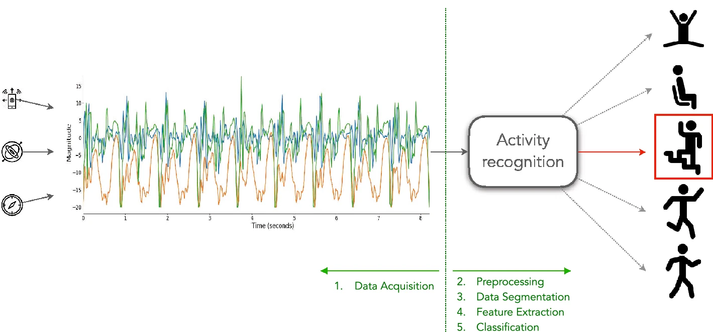
The Human Activity Recognition Using Smartphones dataset is a comprehensive resource for analyzing human activities through smartphone sensor data. Collected from 30 participants aged 19 to 48, the dataset captures six activities:

Walking
Walking Upstairs
Walking Downstairs
Sitting
Standing
Laying

Participants wore a Samsung Galaxy S II smartphone on their waist, which recorded 3-axial linear acceleration and 3-axial angular velocity at a constant rate of 50Hz. The sensor signals underwent noise filtering and were segmented into fixed-width sliding windows of 2.56 seconds with a 50% overlap, resulting in 128 readings per window. From each window, a 561-feature vector was derived, encompassing variables from both time and frequency domains.

This dataset has been widely used in developing and evaluating machine learning models for activity recognition, contributing to advancements in health monitoring, user behavior analysis, and context-aware services.

Human Activity Recognition Dataset Overview

Image From: Trends in human activity recognition using smartphones .

For more details, visit the UCI Machine Learning Repository .

Dimensionality Reduction Methodologies

The effectiveness of GMMs in high-dimensional spaces can be significantly enhanced through dimensionality reduction. This project explores and compares two such techniques: Principal Component Analysis (PCA) and Uniform Manifold Approximation and Projection (UMAP). These methodologies generate low-dimensional representations of the original data, aiming to maintain the essential structure while mitigating the curse of dimensionality. The comparative analysis of these methods is crucial for optimizing the performance of GMMs in human activity recognition tasks.

Importance of Dimensionality Reduction

Dimensionality reduction reduces computational load and enhances model performance by eliminating redundant or irrelevant features. This leads to more efficient training and faster inference times. In the context of the UCI Human Activity Recognition dataset, dimensionality reduction has improved the performance of GMM-based systems by focusing on the most informative features, thereby increasing the accuracy of activity recognition [3] [4].

Impact on Model Performance

Advanced dimensionality reduction techniques, particularly manifold learning methods, play a crucial role in preserving the local geometry of the data. Maintaining this structure is essential for the integrity of the classification information, ensuring that the reduced feature space accurately represents the relationships in the original dataset. This leads to improved clustering and classification outcomes, as the model can more effectively discern between different activity patterns [2] [3].

Preserving Local Geometry

GMM clustering is a fitting method for the UCI Human Activity Recognition dataset because of its ability to handle high-dimensional data, while providing a probabilistic framework for data clustering. Further enhancing the effectiveness of GMMs, dimensionality reduction reduces computational complexity and improves model performance. Consequently, it is a critical step in processing high-dimensional datasets, such as those used in human activity recognition.

Implementation and Results

Data Loading and Preprocessing

The initial phase of this study focused on the meticulous loading and preparation of raw data for subsequent analysis. The procedures implemented are outlined below:

Data Loading: The dataset, consisting of sensor readings recorded during various activities, was loaded from text files using the pandas library. The `load_data` function in `data_loading.py` was employed to consolidate the training and testing datasets into a unified dataframe. This process ensures all data points are available for comprehensive analysis. The function also addresses any duplicated columns by employing a detection and resolution technique.
Missing Value Handling: Prior to modeling, the integrity of the dataset was verified by employing the `detect_missing_values` function from the `data_processing.py` module, supported by the helper function `check_missing`. This step confirms the dataset's completeness with no missing entries, thus ensuring data points are ready for reliable analysis and modeling.
Outlier Management: Potential outliers were identified and addressed using the Interquartile Range (IQR) and Z-score methods, as implemented in the `detect_and_impute_outliers` function. The IQR method, identifying outliers as data points below Q1 - 1.5 * IQR or above Q3 + 1.5 * IQR, and the Z-score method, identifying outliers as values with a z-score greater than 3 or less than -3, were both utilized to gauge the efficacy of each approach. Outliers identified by both methods were imputed using the median value of their corresponding columns. The effects of these methods on the data distribution are visualized through histograms, box plots, and Q-Q plots, which provide a clear comparison between the original and transformed data.

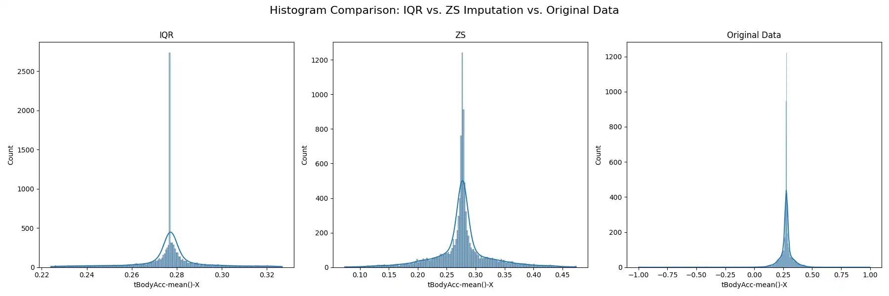
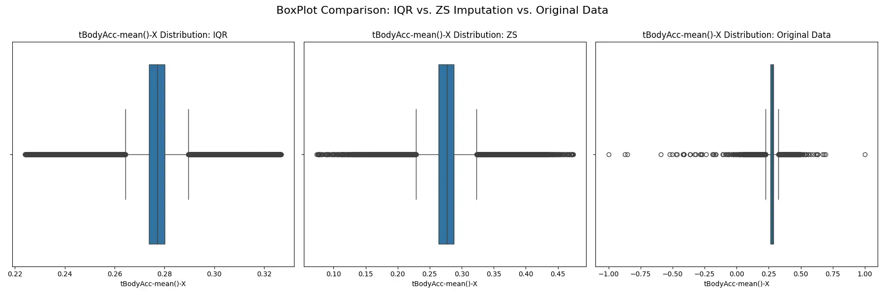
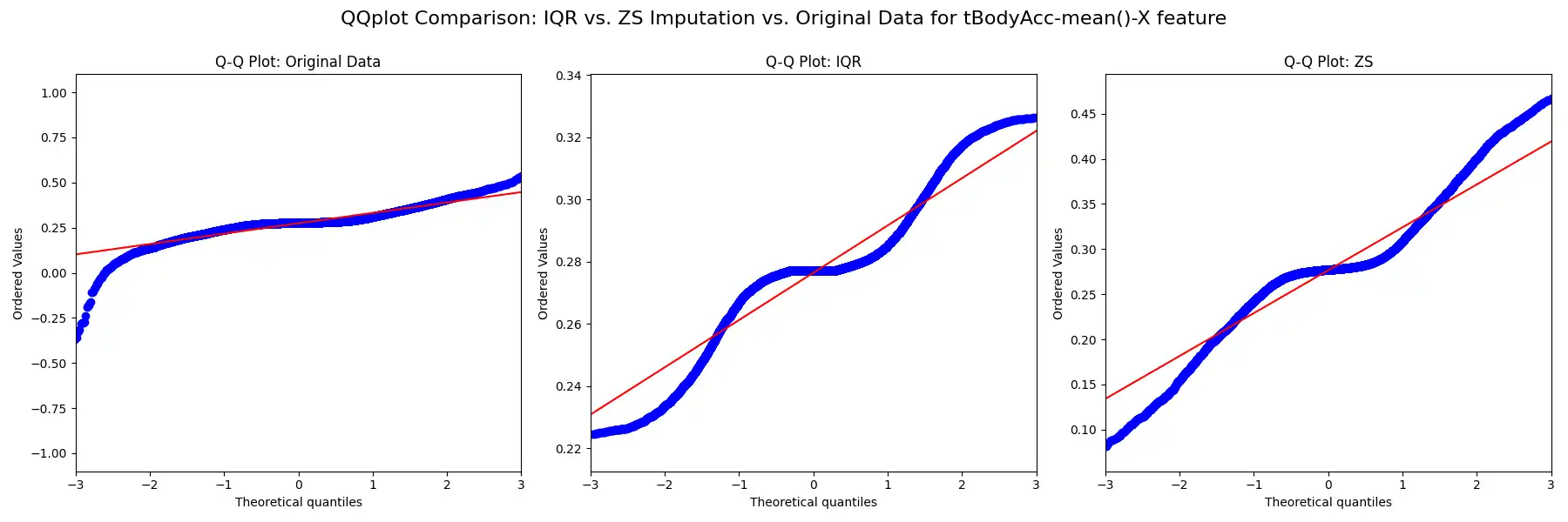
These methodologies ensure the robustness of the dataset against extreme values, which could otherwise skew the results of subsequent clustering processes.

Exploratory Data Analysis (EDA)

The Exploratory Data Analysis (EDA) phase was conducted to gain insights into the dataset’s inherent characteristics. The EDA process, facilitated by the `perform_eda` function in the `eda.py` module, is detailed below:

Subject Distribution: The number of data points contributed by each subject is presented through a bar plot.

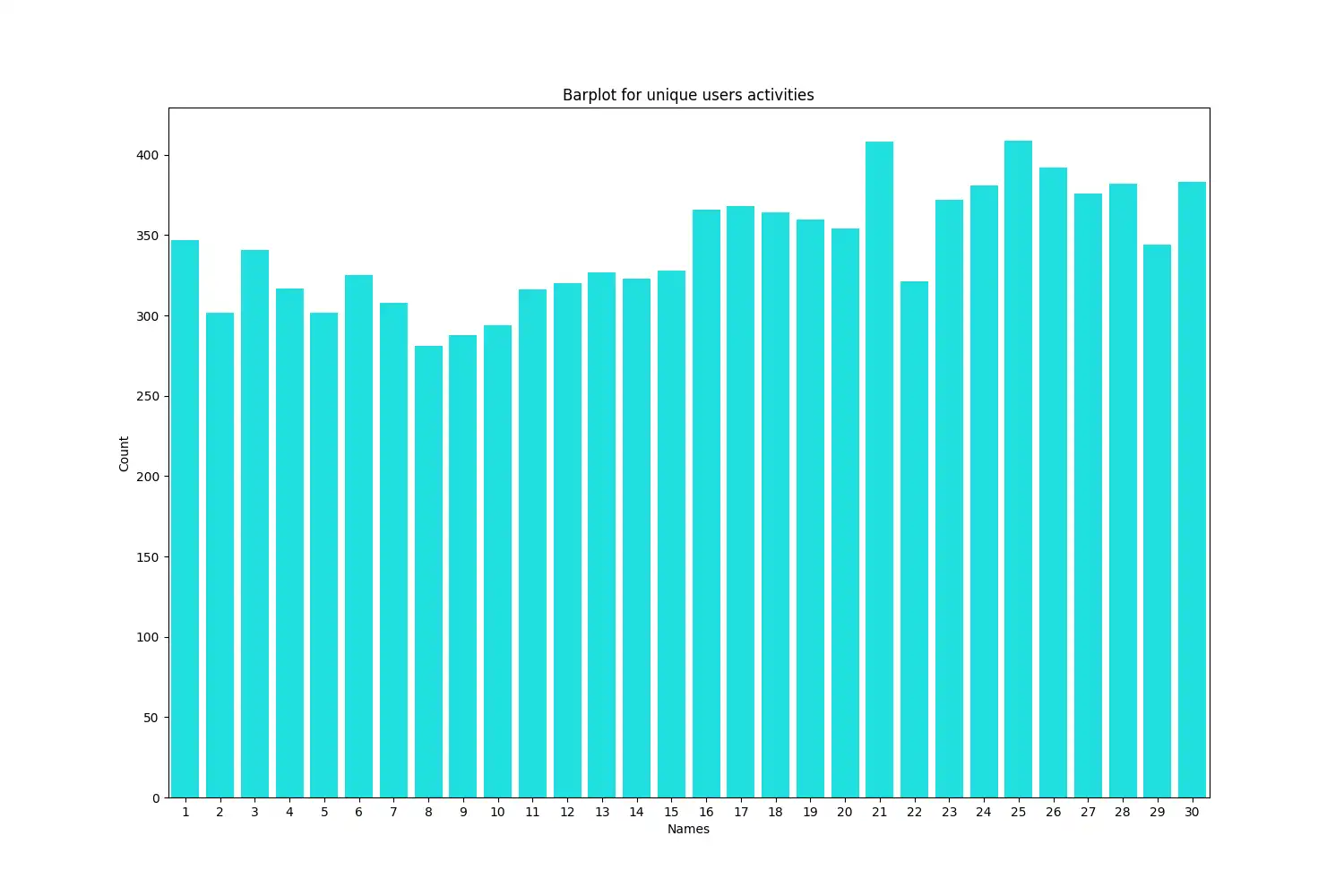
The plot was generated using `seaborn.barplot` to visualize the distribution of unique users and their contribution to the dataset. The counts were sorted in ascending order to clearly visualize the range of data points per subject. This visualization is important in understanding the balance within the dataset.
Activity Distribution: The distribution of activities across subjects was visualized by using `seaborn.countplot`.

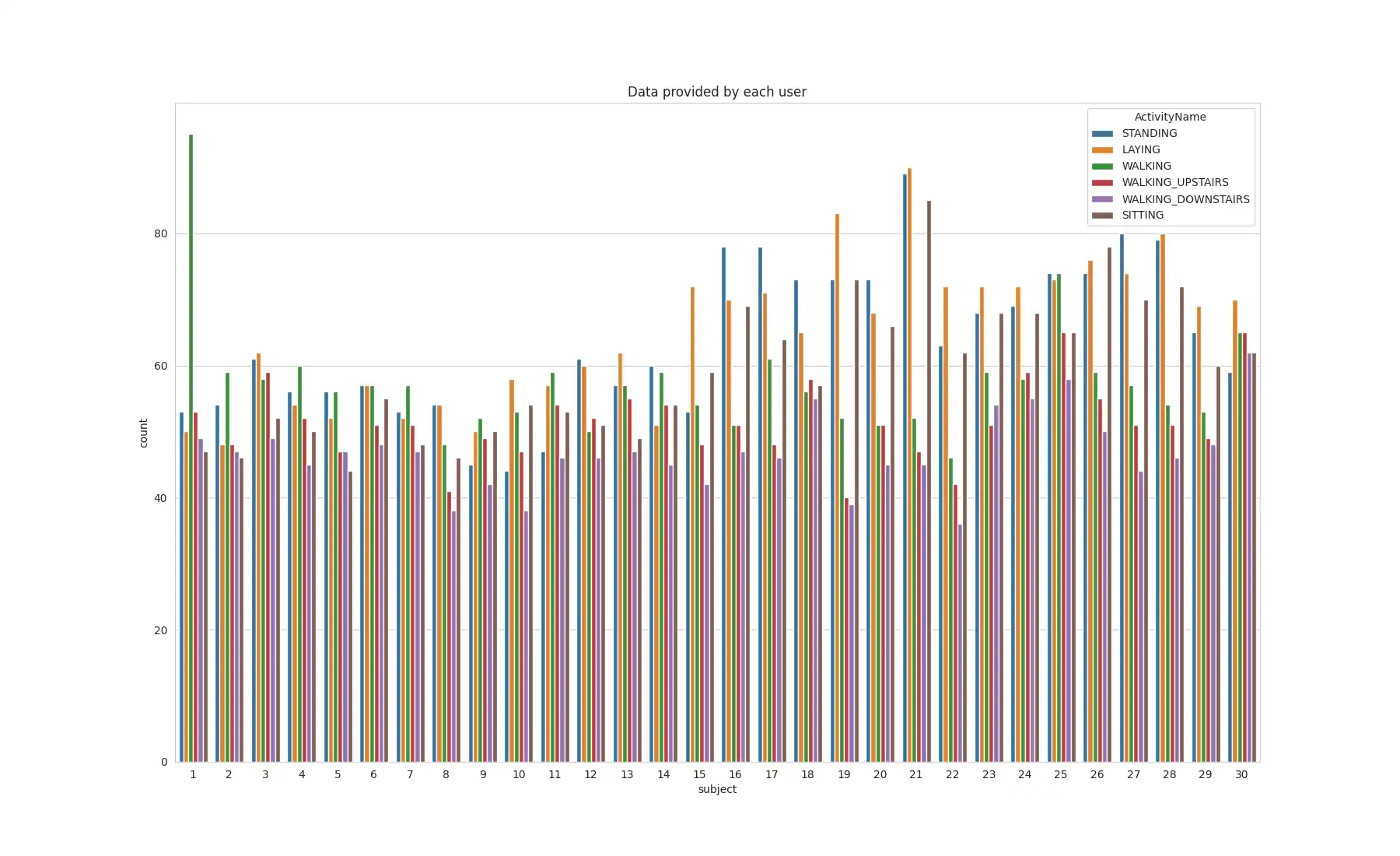
This analysis aims to understand the distribution of each activity per subject, identifying any potential bias or imbalances that may affect the validity of the conclusions drawn from this data.
Stationary Activity Comparison: Stationary activities, such as sitting, standing, and laying, were compared using Kernel Density Estimation (KDE) plots on the 'tBodyAcc-mean()-X' feature.

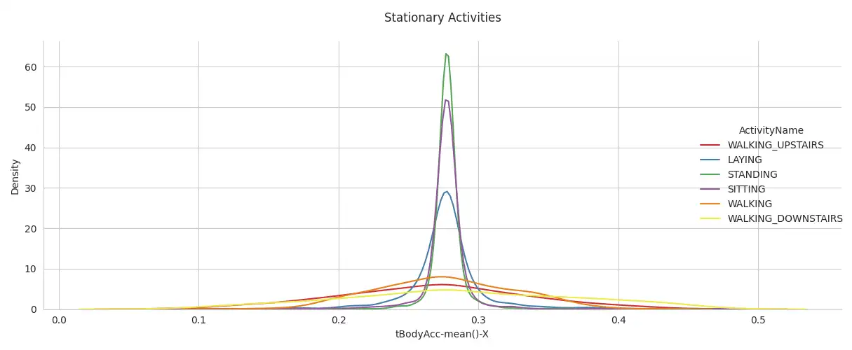
This comparison, facilitated by the use of `seaborn.kdeplot`, provides insight into how different stationary activities are characterized in the dataset by assessing the distribution of these activities based on the 'tBodyAcc-mean()-X' feature.

Feature Engineering

The Feature Engineering stage is focused on preparing the data for subsequent modeling, by implementing scaling and dimensionality reduction techniques.

Feature Scaling: The `feature_scaling` function, based on `StandardScaler` from scikit-learn, was used to scale the features. This step is important to ensure that each feature contributes equally to the model, preventing features with larger scales from dominating those with smaller scales.

UMAP Embedding:

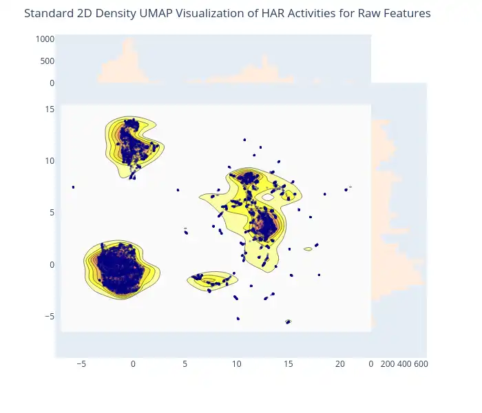
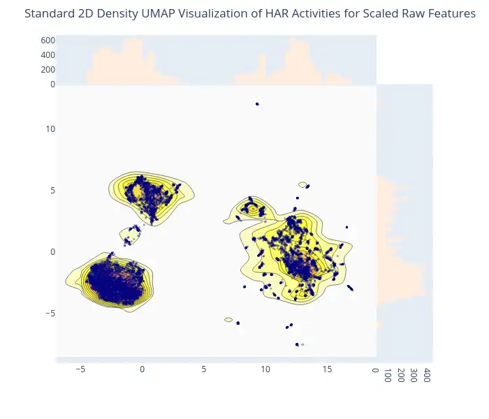
2D Density Plot of Raw Features: The initial application of UMAP before scaling is visualized through an interactive 2D density plot, generated with `plotly.figure_factory.create_2d_density`. This plot provides insights into the distribution of raw features and captures their underlying structure, effectively illustrating how clusters may be formed prior to the scaling process.
2D Density Plot of Scaled Features: An interactive 2D density plot created by Plotly is used to showcase the impact of feature scaling on data distribution. This plot, showing the scaled features after embedding by UMAP, allows for observing how scaling has a notable impact on the separation of clusters, thereby improving data representation.
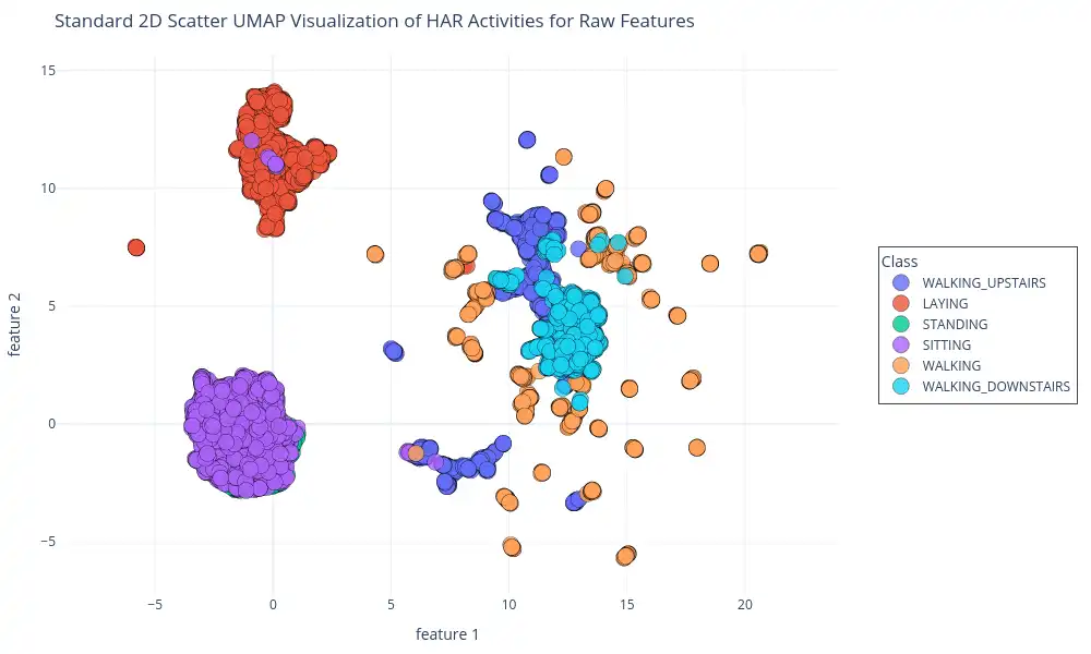
2D Scatter Plot of Raw Features: This plot visualizes the 2D UMAP embedding with data points color-coded by activity class, generated using `plotly.express.scatter`. It helps to validate the clustering observed in the density plots, and also to verify how it aligns with actual classes present in the dataset, and also it provides visual insights into how closely clusters correspond with different activities.

PCA for Dimensionality Reduction:

Variance Ratio Plot: The explained variance ratio by principal component for scaled PCA-transformed features is shown using `matplotlib.pyplot`. This plot displays the individual and cumulative variance ratios for each principal component. This helps to determine the optimal number of components for PCA by balancing dimensionality reduction and information retention. The optimal number of components that explains at least 95% of the dataset variance is highlighted with a vertical dashed line.

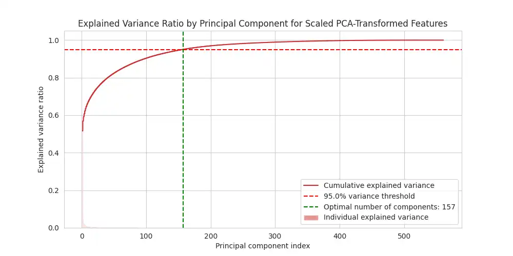
In this study, the analysis indicates that retaining 157 principal components is sufficient to capture 95% of the variance within the dataset, highlighting the effectiveness of PCA for dimensionality reduction. This result was achieved by using `apply_optimal_pca` function in `feature_engineering.py`.

Modeling and Evaluation

The Modeling and Evaluation phase focuses on the application of Gaussian Mixture Models (GMM) for clustering the data, as well as on the assessment of the effectiveness of GMM on dimensionally reduced datasets. The procedures used are:

Determining the Number of Clusters: The optimal number of clusters is identified through analysis of the Bayesian Information Criterion (BIC) and the Akaike Information Criterion (AIC). These values were computed using the `criteria_values` function in `clustering.py` for different number of clusters, with the resulting plots generated by the `plot_criteria_values` function, as shown below. These plots are useful for selecting an appropriate number of clusters for GMM.

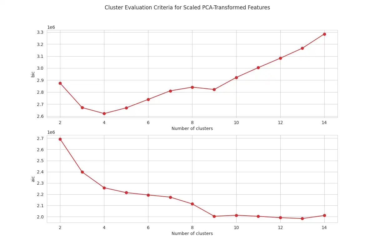
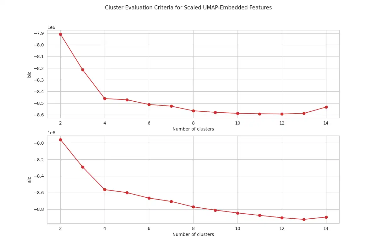
The analysis of the plots for both PCA and UMAP shows that BIC and AIC values decrease sharply up to four clusters, with the rate of decrease slowing down after this point. This analysis suggests that using four components for the GMM is an adequate number for this dataset. The optimal number of components is chosen by looking for the "elbow" point in the curve.
GMM Clustering:
- Clustering on PCA-Transformed Features: This plot shows GMM cluster assignments on data transformed by PCA, using the `perform_gmm_clustering` function. The visualizations of each cluster is generated using `plot_2d_scatter` by mapping the 2D UMAP representation of the data, colored by cluster and labeled with activity class.
  
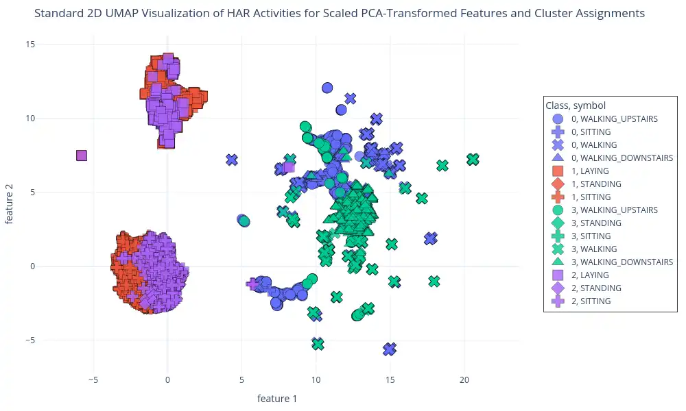
  This plot demonstrates how the GMM algorithm is grouping data points based on a reduced-dimensionality space, and how the GMM derived clusters correlate with known activity labels.
- Clustering on UMAP-Embedded Features: This plot shows GMM cluster assignments on UMAP-embedded data. This visualization, generated using `plot_2d_scatter` function, uses a 2D UMAP representation of the data and is colored based on GMM-assigned clusters. The visualizations show the clusters assigned by the GMM, and also how these clusters correlate with activity labels.
  
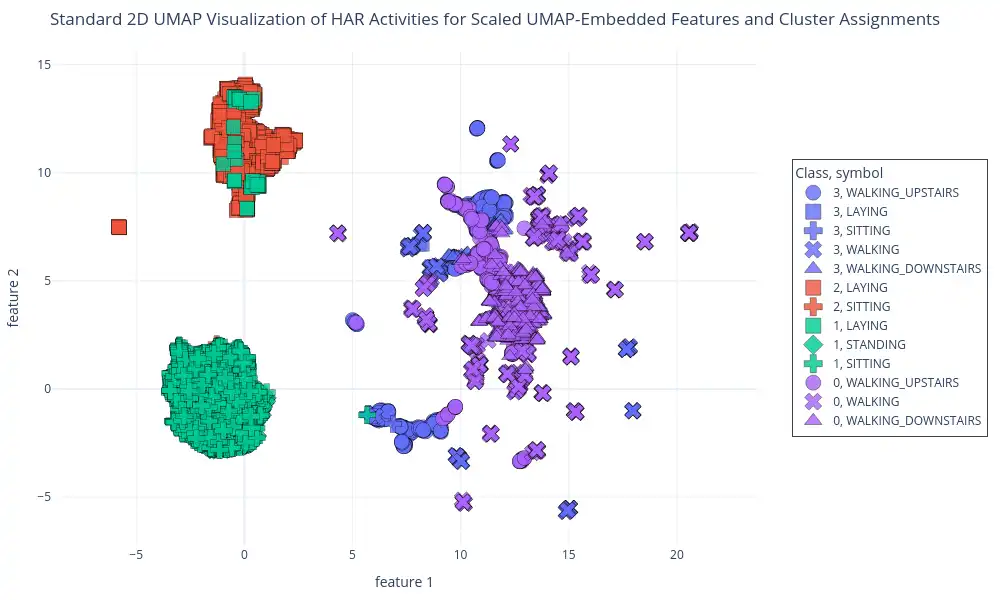
  This visualization displays how the GMM algorithm groups the data points in the dimensionally-reduced UMAP space, and highlights the correlation of these clusters with the given activity labels.

Conclusion

This study has showcased the application of Gaussian Mixture Models (GMMs) for effectively clustering human activity data from the UCI HAR dataset. The impact of dimensionality reduction techniques, such as PCA and UMAP, on the performance of the GMMs was explored. This investigation provides a foundation for further research into employing GMMs for human activity recognition. Furthermore, it highlights the importance of dimensionality reduction for enhancing model performance, computational efficiency, and visual interpretability of GMM clustering through UMAP.

The complete implementation of this project, including source code, documentation, and additional resources, is available in HAR Analysis Project GitHub repository.

Enhanced Human Activity Recognition

Advanced Clustering with Gaussian Mixture Models and Dimensionality Reduction

Table of Contents

References

- Zhao, Y., Shrivastava, A., & Tsui, K. Regularized Gaussian Mixture Model for High-Dimensional Clustering. *IEEE Transactions on Cybernetics*. 2019; 49.
- Popović, B., Janev, M., Krstanović, L., Simić, N., & Delić, V. Measure of Similarity between GMMs Based on Geometry-Aware Dimensionality Reduction. *Mathematics*. 2022
- San-Segundo-Hernández, R., Córdoba, R., Ferreiros, J., & D’Haro, L. Frequency features and GMM-UBM approach for gait-based person identification using smartphone inertial signals. *Pattern Recognit. Lett.*. 2016; 73.
- Chen, Y., Wu, X., Li, T., Cheng, J., Ou, Y., & Xu, M. Dimensionality reduction of data sequences for human activity recognition. *Neurocomputing*. 2016; 210.